
概率门:从比特到概率的电路
Probability gates: from bits to probabilities
逻辑门把电压翻译成 0 和 1,Jev 把用语言描述的世界翻译成概率。本文把 Jev 看作一种「概率门」,参考随机计算、贝叶斯网络和概率比特的已有工作,讨论可以用它组合出哪些元件,以及怎样用这些元件搭一个世界模拟器。
Logic gates turn voltages into 0 and 1; Jev turns a description written in language into probabilities. This post treats Jev as a "probability gate", draws on prior work in stochastic computing, Bayesian networks and probabilistic bits, and looks at which components can be built from it and how they could form a world simulator.
电路里流动的是电子,逻辑门把它翻译成 0 和 1。0 和 1 可以组合、堆叠,于是有了计算机。
Jev 里流动的是 token,它把一段文字描述翻译成概率。概率也可以组合、堆叠,规则就是概率论。那么,大量 Jev 组合起来,能不能成为一种新的电路?
Jev 是 TypeSafe AI 在 9 月发布的模型。它不生成文字,只回答三类问题:是或否、多选一、打分,每个答案都是一个概率分布。官方给出的单次调用耗时是 70–500 毫秒,价格比前沿大模型低几十到几百倍。
为什么不是逻辑门
我最初的类比是晶体管和逻辑门。细想之后,这个类比有点牵强,原因有两个。
第一,逻辑门是「比特进、比特出」,输出和输入是同一种东西,所以可以无限串联。Jev 是「文本进、概率出」。
第二,也是更根本的:布尔逻辑只看各自的值就能组合,A 且 B 的真假只取决于 A 和 B 各自的真假。概率不行。只知道 P(A) = P(B) = 0.7,P(A 且 B) 可以是 0.4 到 0.7 之间的任何值,取决于 A 和 B 有多相关。要组合,就必须知道依赖关系:
P(A 且 B) = P(A) × P(B | A)
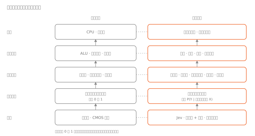
所以更准确的名字是概率门:给定一段用语言描述的输入 X,输出少数几种结果 Y 的概率分布,数学上就是条件概率 P(Y | X)。Jev 是概率门的一种实现;大模型加校准、专门训练的小分类器也可以是。这和数字电路里同一种门可以用 TTL 或 CMOS 实现类似:实现方式不同,速度、成本和精度也不同。
这个定义有理论依据。Cox 在 1946 年证明、Jaynes 后来系统阐述过:在几条关于一致推理的基本假设下,处理不完整信息的规则只能是概率论。当概率只取 0 和 1,概率论就退化成布尔代数。逻辑电路是概率电路的特例。
前人走过的三条路
把概率当作电路里的信号,并不是新想法。至少有三条相关的研究路线。
随机计算(1960 年代)。用一串随机比特表示一个概率,其中 1 所占的比例就是概率值。一个与门就能做概率乘法,一个多路选择器就能做加权加法。前提是输入之间相互独立:两路输入一旦相关,乘法结果就不对。这和我之前做的一个模拟一致:平均 70% 准确的判断者投票,错误互不相关时 27 票就能到 98.5%;相关性为 0.2 时,243 票也只到 81.6%。组合概率时,必须同时考虑它们之间的相关性。
贝叶斯网络(1980 年代,Pearl)。用一张有向图表示变量之间谁依赖谁,每个节点挂一张条件概率表。代数完全正确,却没能普及,卡在数字从哪里来:几百个变量、几千条条件概率,要请专家一条条手填。这就是当年专家系统的「知识获取瓶颈」。Jev 可以解决这个问题:任何能用语言描述的条件概率,都能在零点几秒内、以很低的成本得到一个估计值。
概率比特(2017 年起)。研究者用会随机翻转的器件搭电路,每个单元以由输入决定的概率输出 1。这样搭出的电路有一个逻辑电路没有的性质:可以反向推断。把一个乘法电路的输出固定住,它会在可能的因数之间来回涨落,相当于做了因数分解。原因在于,概率电路表示的是一个联合分布,固定哪一端,就能推断另一端。
总结一下:概率电路的代数和组合规则早已成熟,主要问题也已经清楚。过去缺少的,是一个便宜、通用、可以用语言配置的概率来源。
用概率门组合出更高阶的元件
数字电路从门出发,组合出加法器、多路选择器、触发器,再到运算单元和处理器。概率门也可以这样往上搭。下面这些元件,都只由 Jev 调用加普通代码组成:
| 元件 | 组成 | 对应的电路 | 作用 |
|---|---|---|---|
| 差分门 | 同时问「是 X 吗」和「不是 X 吗」,合并为(是 + 1 − 不是)÷ 2 | 差分放大器 | 抵消「倾向回答是」这类共模偏差;两个答案之和偏离 1,说明问题本身没问好 |
| 一致性恢复器 | 对一组相关命题分别提问,再投影到离它最近的一致分布 | 电平恢复 | 把一组判断修正到满足概率公理 |
| 条件概率表 | 把父节点的每种取值分别写进输入,同一层并行提问 | FPGA 查找表 | 按需生成贝叶斯网络中一个节点的条件概率 |
| 证据融合器 | 在先验的对数几率上,加上每路证据的对数似然比,按估计的相关性打折 | 加法器 | 防止同一条证据或同一个先验被重复计算 |
| 信念寄存器 | 保存某个假设的概率,每来一条证据,用似然比做一次贝叶斯更新 | 寄存器、积分器 | 保存当前对某个假设的判断 |
| 反演器 | 对每个候选原因问「如果是它,会看到这个现象吗」,乘以该原因的先验概率,再归一化 | 可逆电路 | 从结果推原因:诊断、归因 |
| 三态门 | 概率落在不确定区间时输出「不知道」 | 三态缓冲器 | 把这一单交给人或大模型 |
| 迟滞门 | 超过 0.7 才置位,低于 0.3 才复位 | 施密特触发器 | 防止结论在阈值附近来回跳 |
| 采样器 | 按概率掷骰子,随机种子固定 | 随机源 | 根据概率生成一次具体结果,并且可以复现 |
| 校准器 | 用真实结果修正门的输出 | 微调电路 | 让门给出的概率对得上现实里的频率 |
其中有三样,对应的电路器件只是形式相近,做的事情不同:
- 反演器:可逆电路的输入和输出一一对应,可以原样倒推;反演器面对的是多个可能的原因,要结合每个原因的先验概率,算出它们各自的可能性;
- 三态门:三态缓冲器的高阻态表示「不驱动这条线」;三态门输出的「不确定」是一个判断结果,交给人或大模型处理;
- 一致性恢复器:数字电路的电平恢复靠增益,每一级都把误差压掉,所以几十亿个门串起来也不会累积误差。一致性恢复器只能去掉相互矛盾的那部分误差。Predd 等人(2009)证明,把不一致的概率投影到一致集合上,结果在 Brier 分数上严格优于原值;但如果一组判断朝同一个方向偏,投影之后仍然是错的。所以概率电路更像模拟电路:误差会逐级累积,能搭多深取决于误差预算。
再往上:处理单元
这些元件再组合,可以得到四种处理单元:
- 推断单元:条件概率表 + 证据融合 + 信念寄存器,回答「现在最可能是什么情况」;
- 诊断单元:反演器 + 信念寄存器,再加一个「下一问问什么」的选择器,挑出最能缩小不确定性的问题;
- 预测单元:条件概率表 + 一致性恢复 + 校准,回答「接下来发生 X 的概率是多少」;
- 模拟单元:把预测单元接成一个循环,就是世界模拟器。
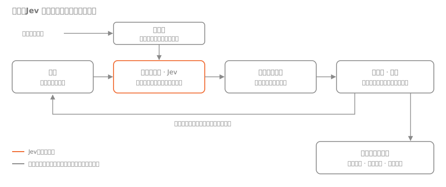
每个时钟周期,先由大模型或人根据当前状态的文字描述,列出下一步可能发生的候选事件;Jev 给出这些事件的概率;一致性恢复器把这组概率修正到相互一致;采样器按概率抽取这一步实际发生的事件;结果写回状态,进入下一步。重复上万次,就得到结果的分布。
前文说的相关性在这里同样成立:分别问每个事件的概率、再分别采样,等于假设同一步里的事件相互独立。要保留相关性,可以把互斥的结果组合写成一个多选题一次问完,或者按链式法则逐个采样:先抽第一个事件,把结果写进输入,再问下一个事件的条件概率。后者更准,但请求数会成倍增加。
它和「让大模型扮演一群人去生成行为」的社会模拟有一个关键区别:概率和随机性分开了。概率由 Jev 给出,可以校准、可以审计;随机由代码产生,可控、可复现。成本也低到可以真正跑上万条轨迹。粗算一下:1 万条轨迹 × 50 步,如果每步用一次请求同时问 20 个事件,约 50 万次请求;按每次约 1,000 个输入 token、网关公布的每百万输入 token 0.042 美元计算,约 21 美元。改用逐个条件采样,请求数还要乘以事件数。
在模拟单元之上再加一层决策:比较不同选项下的结果分布,看最坏情况,看哪些变量最敏感。很多现实系统对初始条件敏感,无法预测具体结果,但可以估计结果的分布。
边界
这个类比也有几处限制:
- 概率的形式对,数值未必对。Jev 的概率是它自己的估计,按它的训练数据校准;世界模型需要和现实中的发生频率一致。没有用真实结果校准,模拟结果就没有预测意义。
- 结构比参数更难。变量选错、依赖关系画错,比单个概率不准影响更大。
- 「已知」不等于「如果」。「已知我换了工作」和「如果我去换工作」是两个不同的概率。决策需要的是后者,Jev 能不能区分,要实测。
- 模拟的范围取决于候选事件和描述。Jev 不生成文字,下一步可能发生什么,要由大模型或人列出来;没有列进候选、没有写进描述的因素,模拟不会考虑。
- 长期结果仍然难以预测。即使每个概率都对,时间越长,结果的分布也越分散。模拟能告诉我们分布和敏感变量,不能给出确定的结局。
所以我的判断是:Jev 不是布尔计算里的晶体管,但它可能是第一个便宜到可以大量调用的概率推理元件。如果这一点成立,过去因为成本太高而没能普及的概率推理方法,可能会重新变得实用。
接下来
我们会用真实的 Jev 验证这些设想:
- 差分门:正反双问是否比单问更准、更校准。语言模型处理否定句本身容易出错,「不是 X 吗」的误差未必是共模的,所以要分开测试改写成否定句和交换「是」「否」定义两种问法;
- 相关性:换问法、拆证据、换模型之后,错误之间还剩多少相关;
- 一致性恢复:分别问 P(A)、P(B)、P(A 且 B) 等,统计违反概率公理的比例,看恢复之后预测是否更准;
- 前瞻预测:在 Jev 发布之后才揭晓结果的公开预测题上,现在登记 Jev 给的概率,等结果出来再算准确度和校准度。用来检验 Jev 的概率和真实频率是否一致,并对照同一道题的预测市场价格和前沿大模型的回答;
- 小型世界模拟:在有历史结果数据的场景里,看模拟出的分布与真实频率是否吻合。
结果出来后,再写一篇。
说明:文中关于 Jev 的数字来自 TypeSafe AI 官方和第三方网关的公开资料。作者和榫卯 Tenon AI 与 TypeSafe AI 没有合作关系,也没有收到任何费用。
Electrons flow through a circuit, and logic gates turn them into 0 and 1. Zeros and ones can be combined and stacked, and that gave us computers.
Tokens flow through Jev, and it turns a written description into probabilities. Probabilities can also be combined and stacked; the rules are probability theory. So can a large number of Jev calls, wired together, become a new kind of circuit?
Jev is a model TypeSafe AI released in September. It does not generate text. It answers three kinds of questions: yes or no, pick one of several options, and a score on a scale. Every answer is a probability distribution. According to the company, a call takes 70–500 ms and costs tens to hundreds of times less than a frontier language model.
Why it is not a logic gate
My first analogy was the transistor and the logic gate. On reflection, it does not quite fit, for two reasons.
First, a logic gate takes bits in and puts bits out. Input and output are the same kind of thing, so gates can be chained indefinitely. Jev takes text in and puts probabilities out.
Second, and more fundamentally, Boolean logic composes from values alone: whether A AND B is true depends only on whether A and B are each true. Probabilities do not work that way. Knowing only P(A) = P(B) = 0.7, P(A and B) can be anything from 0.4 to 0.7, depending on how correlated A and B are. To combine them you need the dependency:
P(A and B) = P(A) × P(B | A)
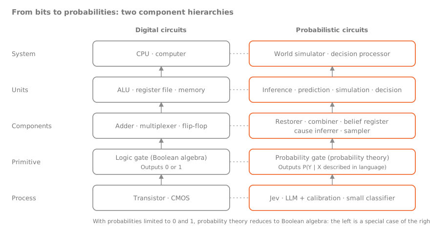
A more accurate name is probability gate: given an input X described in language, it outputs a probability distribution over a few outcomes Y. Mathematically it is the conditional probability P(Y | X). Jev is one implementation; a language model plus calibration, or a small trained classifier, can be another. This is similar to how the same digital gate can be built in TTL or CMOS: different implementations, with different speed, cost and accuracy.
The definition has a theoretical basis. Cox proved in 1946, and Jaynes later set out in detail, that under a few basic assumptions about consistent reasoning, the rules for handling incomplete information have to be probability theory. When probabilities are restricted to 0 and 1, probability theory reduces to Boolean algebra. Logic circuits are a special case of probabilistic circuits.
Three earlier lines of work
Treating probabilities as signals in a circuit is not a new idea. There are at least three related lines of research.
Stochastic computing (1960s). A probability is represented by a stream of random bits, where the share of 1s is the value. A single AND gate multiplies two probabilities, and a multiplexer computes a weighted sum. This only works if the inputs are independent: once two input streams are correlated, the product is wrong. It matches a simulation I ran earlier: with voters who are 70% accurate on average, 27 votes reach 98.5% when their errors are uncorrelated; with a correlation of 0.2, even 243 votes only reach 81.6%. When you combine probabilities, you have to account for how they are correlated.
Bayesian networks (1980s, Pearl). A directed graph records which variables depend on which, and each node holds a conditional probability table. The algebra is correct, yet the approach never became common. It got stuck on where the numbers come from: hundreds of variables and thousands of conditional probabilities had to be filled in by experts, one by one. This was the "knowledge acquisition bottleneck" of expert systems. Jev can address it: any conditional probability that can be described in language can be estimated in a fraction of a second at very low cost.
Probabilistic bits (since 2017). Researchers build circuits from devices that flip at random, where each unit outputs 1 with a probability set by its inputs. Such circuits have a property logic circuits lack: they can infer in reverse. Fix the output of a multiplier circuit, and it fluctuates between possible factors, which amounts to factoring the number. The reason is that a probabilistic circuit represents a joint distribution; fix either end and you can infer the other.
In short, the algebra and composition rules of probabilistic circuits have been settled for a long time, and the main problems are known. What was missing was a cheap, general source of probabilities that can be configured in language.
Building higher-level components from probability gates
Digital circuits start from gates and build adders, multiplexers and flip-flops, then arithmetic units and processors. Probability gates can be built up the same way. Each component below uses only Jev calls and ordinary code:
| Component | How it is built | Circuit counterpart | Purpose |
|---|---|---|---|
| Differential gate | Ask "is it X?" and "is it not X?" together and combine them as (yes + 1 − no) ÷ 2 | Differential amplifier | Cancels common-mode bias such as a tendency to answer yes; if the two answers do not sum to about 1, the question itself is poorly posed |
| Coherence restorer | Ask about a set of related propositions separately, then project onto the nearest consistent distribution | Level restoration | Corrects a set of judgments so they satisfy the probability axioms |
| Conditional probability table | Write each value of the parent nodes into the input and ask in parallel within one layer | FPGA lookup table | Produces a node's conditional probabilities in a Bayesian network on demand |
| Evidence combiner | Start from the prior log-odds and add the log-likelihood ratio of each piece of evidence, discounted by their estimated correlation | Adder | Prevents the same evidence, or the same prior, from being counted twice |
| Belief register | Holds the probability of a hypothesis and applies a Bayesian update with the likelihood ratio of each new piece of evidence | Register, integrator | Keeps the current judgment about a hypothesis |
| Cause inferrer | For each candidate cause, ask "if this were the cause, would we see this?", multiply by that cause's prior probability, and normalize | Reversible circuit | Infers causes from results: diagnosis and attribution |
| Tri-state gate | Outputs "unknown" when the probability falls in an uncertain band | Tri-state buffer | Hands the case to a person or a larger model |
| Hysteresis gate | Sets above 0.7 and resets below 0.3 | Schmitt trigger | Stops a conclusion from flipping back and forth near the threshold |
| Sampler | Draws an outcome according to the probabilities with a fixed random seed | Random source | Produces one concrete outcome from a probability, reproducibly |
| Calibrator | Corrects a gate's outputs against real outcomes | Trimming circuit | Makes the gate's probabilities match real-world frequencies |
For three of these, the circuit counterpart only looks similar; the job is different:
- Cause inferrer: in a reversible circuit, inputs and outputs map one to one, so you can step back exactly. A cause inferrer faces several possible causes and has to combine each one's prior probability to work out how likely each is.
- Tri-state gate: a tri-state buffer's high-impedance state means "not driving this line". A tri-state gate's "uncertain" is a judgment, passed to a person or a larger model.
- Coherence restorer: level restoration in digital circuits relies on gain, which removes the error at every stage, so billions of gates can be chained without errors building up. A coherence restorer only removes the part of the error that is self-contradictory. Predd et al. (2009) proved that projecting incoherent probabilities onto the coherent set gives a result that is strictly better under the Brier score; but if a set of judgments is biased in the same direction, it is still wrong after the projection. Probabilistic circuits are therefore closer to analog circuits: errors build up stage by stage, and how deep a circuit can go depends on the error budget.
One level up: processing units
Combining these components gives four processing units:
- Inference unit: conditional probability tables + evidence combiner + belief register; answers "what is most likely going on now?"
- Diagnosis unit: cause inferrer + belief register, plus a selector for the next question that picks the one that most reduces uncertainty.
- Prediction unit: conditional probability tables + coherence restoration + calibration; answers "what is the probability that X happens next?"
- Simulation unit: a prediction unit connected in a loop, which is a world simulator.
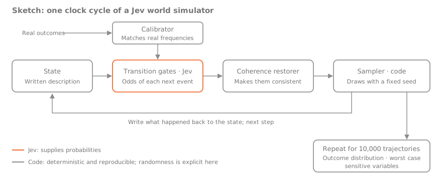
In each clock cycle, a language model or a person first lists the candidate events that could happen next, based on the written description of the current state. Jev gives the probabilities of those events. The coherence restorer makes those probabilities consistent with each other. The sampler draws the events that actually happen in this step, and the result is written back to the state for the next step. Repeating this ten thousand times gives a distribution of outcomes.
The point about correlation from earlier applies here too: asking for each event's probability and sampling each one separately assumes the events in a step are independent. To keep the correlation, you can write the combinations of mutually exclusive outcomes as one multiple-choice question, or sample one event at a time with the chain rule: draw the first event, write the result into the input, then ask for the next event's conditional probability. The second approach is more accurate but multiplies the number of requests.
This differs in one important way from social simulations in which a language model plays a group of people and generates their behavior: probability and randomness are separated. Jev supplies the probabilities, which can be calibrated and audited; code supplies the randomness, which is controllable and reproducible. The cost is also low enough to actually run ten thousand trajectories. A rough estimate: 10,000 trajectories × 50 steps, with one request per step asking about 20 events at once, is about 500,000 requests. At roughly 1,000 input tokens per request and the gateway's listed price of $0.042 per million input tokens, that is about $21. Sampling events one at a time multiplies the request count by the number of events.
A decision layer can sit on top of the simulation unit: compare the outcome distributions of different options, look at the worst cases, and see which variables matter most. Many real systems are sensitive to initial conditions, so their specific outcomes cannot be predicted, but the distribution of outcomes can be estimated.
Limits
The analogy has several limits:
- The form of the probabilities is right; the numbers may not be. Jev's probabilities are its own estimates, calibrated on its training data. A world model needs them to match how often things happen in reality. Without calibration against real outcomes, the simulation has no predictive value.
- Structure is harder than parameters. Choosing the wrong variables or drawing the wrong dependencies matters more than an individual probability being off.
- "Given" is not the same as "if". "Given that I changed jobs" and "if I change jobs" are two different probabilities. Decisions need the second; whether Jev can tell them apart has to be tested.
- What the simulation covers depends on the candidate events and the description. Jev does not generate text, so a language model or a person has to list what could happen next; anything left out of the candidates or the description is not considered.
- Long-term outcomes remain hard to predict. Even if every probability is right, the distribution spreads out over time. A simulation can show the distribution and the sensitive variables, not a definite ending.
So my view is this: Jev is not the transistor of Boolean computing, but it may be the first probabilistic reasoning component cheap enough to call in large numbers. If that holds, probabilistic reasoning methods that never caught on because they were too expensive may become practical again.
Next
We will test these ideas with the real Jev:
- Differential gate: whether asking both ways is more accurate and better calibrated than asking once. Language models are prone to errors with negation, so the error on "is it not X?" is not necessarily common-mode; the experiment has to test negated wording and swapped yes/no definitions separately.
- Correlation: how much correlation remains between errors after changing the wording, splitting the evidence or switching models.
- Coherence restoration: ask for P(A), P(B), P(A and B) and so on, count how often the answers violate the probability axioms, and check whether predictions improve after restoration.
- Forward forecasting: on public forecasting questions that resolve after Jev's release, record Jev's probabilities now and score accuracy and calibration once the results are in. This checks whether Jev's probabilities match real frequencies, compared with prediction-market prices and frontier language models on the same questions.
- Small world simulation: in settings with historical outcome data, check whether the simulated distribution matches the real frequencies.
I will write a follow-up when the results are in.
Note: the figures about Jev come from TypeSafe AI and third-party gateways' public material. The author and Tenon AI have no business relationship with TypeSafe AI and have received no payment.